Christina O'Malley, PhD

Introduction and Objective

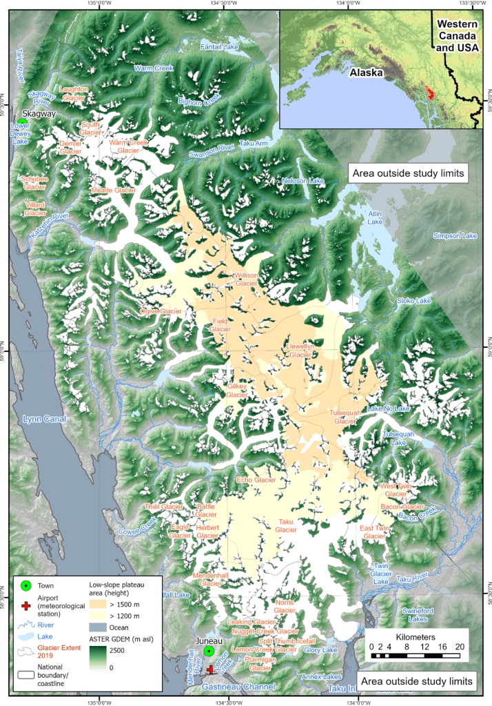
The Alaskan Ice Field is the third largest in the world after the Greenland and Antarctic ice sheets, and the Juneau Ice Field is one of the most studied, due to its relative accessibility. In addition to size, these glaciers are uncharacteristically low in elevation, which makes them more sensitive to to small local climatic changes. The combination of volume and potential to have a summer melting period mean that these glaciers are a significant contributor to sea level rise, and need to be understood (Davies, 2021).

The JIRP Mission is to provide an authentic experience for students to participate in active research in the Juneau Ice Field near Juneau, Alaska. Students and scientists come from across the world to learn not only geology and glaciology, but also wilderness survival. This program has been active for sixty years and produced generations of glacial and climate scientists (Juneau Icefield Research Program).

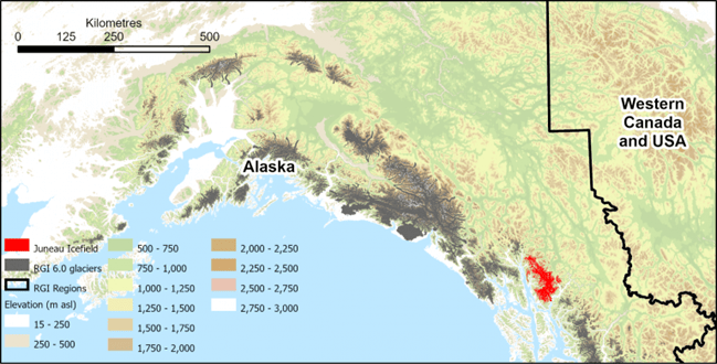
In the summer of 2023, researchers connected to the Juneau Icefield Research Project (JIRP) began to observe that glacial lakes were forming from meltwater earlier and faster than in prior years (Fortner, personal communication). Glacial lakes form over the summer as the snow in the icefield melts (in the northern hemisphere, between the last snow in late April and the first snows in October). Water frequently flows downhill or through crevasses to streams and rivers that head to the ocean, but sometimes water is trapped at elevation in pools of ice. The formation of these lakes, because the meltwater stays in place and doesn’t drain away, are a visible indicator that the climate of an area has changed. When the timing of these lakes or the rate of their growth is earlier in the season than usual, it is an indication that the sum of the change of climactic factors may be significant.

My question: Taku Glacier is the largest glacier in the Juneau Ice Field near Juneau,
Alaska. Over time, this glacier has been monitored by the Juneau Icefield Research Program, and in the last summer season, researchers reported that glacial lakes may be forming more quickly than in past years. This project will streamline identification of glacial extent change using Landsat data and identify potential sites for the growth of Glacial Lakes in the 2023 summer season. Awareness of these locations can lead to more focused research (by satellite data, or fieldwork) to the locations and extent of the growth of these meltwater lakes.

Data Collection and Management

Data for this project was sourced from the Earth Explorer website managed by the
United States Geological Survey (USGS). This study focused on the Taku Glacier at 58.5950° N, 134.1797° W (entered Earth Explorer as 58.5950, -134.1979). Data from the LandSat 8-9 Operational Land Imager (OLI). Bands 3, 5, and 6 are able to gain data about water on the surface, and so those layers were downloaded as TIF files for this analysis, with QA_Pixel data files for the attempted cloud analysis of the same dates. Details about the metadata attached to these files is described in Table 1. Raw data was not corrected for the presence of clouds.

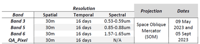
In order to assess changes with snow and ice melt over the summer months, data was selected from Earth Explorer after filtering for low clouds (10% or less). First, images from April and May were checked to identify a “before” image. Late April is when the Taku Glacier reaches its largest volume/extent, (when the glacier has its largest volume/extent). Images from August and September were assessed for the “after image”, as the snows start falling usually by October, not only adding snow back to the icefield but obscuring the image with thick clouds. The date of 09 May 2023 was chosen for having the clearest view of the glacier in the spring, and 05 September 2023 was selected as the late summer “after” date.

Methodology

Data for this study was downloaded from the USGS EarthExplorer as TIF files, and did not require more processing before accessing with ArcGIS Pro. The data was put into multiple Maps in a single project, according to Band, so that each band could be processed separately. This study focused on the Taku Glacier at 58.5950°N, 134.1797°W using data from the LandSat 8-9 Operational Land Imager (OLI) Data for this analysis was downloaded for the selected bands from EarthExplorer (USGS) as described above. A map was created for each band, containing the data for both dates for each band.

Band Selection
Three bands were chosen due to the variety of measurements they would cover, with the goal of identifying areas where a change in ice and snow cover had occurred. Those bands were:

• Band 3 measures the Green wavelengths of light, which identifies peak vegetation growth. When Ice and snow is present, band 3 would return a low value due to low vegetation. As this study spans the summer months, as the snow and ice melt and plants grow in their place, this value is expected to increase. The change over time in this band would then illustrate places where the ice and snow not only melted away, but plants would grow (Loyd, 2013).
• Band 5 measures wavelengths in the Near Infrared (NIR) range, and indicated turgidity or rigidity in plants (sometimes considered “plant health”). This would give an indication of not only locations with plant growth (and thus, low ice and snow coverage) but also locations where there was enough water that plants were not wilting (Loyd, 2013).
• It is worth considering that there is an inherent relationship between Band 3 (Green) and Band 5 (NIR). Both indicate vegetative growth, and give clues to the presence of ice and snow; Band 5 further gives clues about the abundance of water.
• Band 6 measures short wave infrared radiation: heat. This band is encouraged in many geological applications, and in fact, stony places will absorb heat from the environment and radiate it back out, where it can be detected. In this analysis, Band 6 is most dissimilar (compared to Bands 3 and 5) as it is detecting radiant energy rather than reflected energy. In relation to the icefield, as ice and snow melt, they leave behind terrain that can achieve a temperature above that of the temperature of the frozen water (as all energy first goes to phase change of the water before it can go to warming the environment), which is why we see the pattern of no change (or nearly no change) in the snow and ice covered areas for Band 6 once the analysis is completed (Loyd, 2013).

Strategies to Manage Errors Due to Cloud Cover in the Data
During this project I attempted to remove the error in the data due to clouds in several
ways, as described below:

• Combine multiple Raster datafiles together using a raster tool. The rationale for this technique is that clouds exist in different places on different days, so if you combine data from different days, ultimately you’ll end up with data representing the whole. For many studies, this probably works – but for me, combining data from multiple days (when the Earth Explorer often had gaps between data that met my 20% cloudcover filter) meant losing some of the accuracy of the location of the ice in the icefield.
• Remap from the Raster Function pane was also a possible solution, but I could not find the correct sequence of buttons and it did not turn up in any of the ArcGIS search tools.
• Using Clip to create “no data” data in the raster file where the clouds are to remove those cells from the dataset, by removing cells indicated to contain clouds using the QA_Pixel dataset. Ultimately, this led to a map product after comparing for differences where the product was visually similar to using the raster that just had clouds included.
• After reading some primary literature about what researchers were using to track glaciers and meltwater, I decided instead that the best solution (for this project) would be to go back to Earth Explorer and see if there was relatively cloudless data in the correct date ranges. I reset my parameter for cloudcover to 10% (I also tried 5%, but didn’t get results in ranges that were viable for addressing the research question), and visually assessed the location of the clouds in the sample images, and chose days where the clouds that were in the images were of the least impact to the Taku Glacier Icefield.

Summary: while it would have been more satisfying, I think, so have been able to use data that I cleared the clouds from myself, I was happy with this solution because it gave me a high quality product that still accurately illustrated the changes in the data.

Determining the Amount of Change between Datasets
For this dataset, both ArcMap and ArcGIS Pro were used to assess the change in the
datasets. Ultimately, ArcGIS Pro was settled on simply because it was faster and simpler to move the data to the correct folders (as access to ArcMap was on a remote machine). The Change Detection Wizard in ArcGIS Pro was used to identify the pixel value change, that is, the differences between data collected on the two dates. The analysis was performed using the absolute difference type, and Single Band Difference Method. For this analysis, the change histogram was used to filter out the portion of the data where clouds indicated an unusually large change. (At these wavelengths, the water in clouds had different reflectance than water held in ice and snow in the icefield. Therefore, the difference was greatest in the small part of the map with clouds, and this provided a simple but seemingly effective way to remove the clouds from the analysis). The analysis was run with and without this modification using the histogram, and the difference in the maps correlated with the location of the clouds. The three bands were combined into a single map using the Combine (Spatial Analyst Tool), in order to summarize the results.

Results

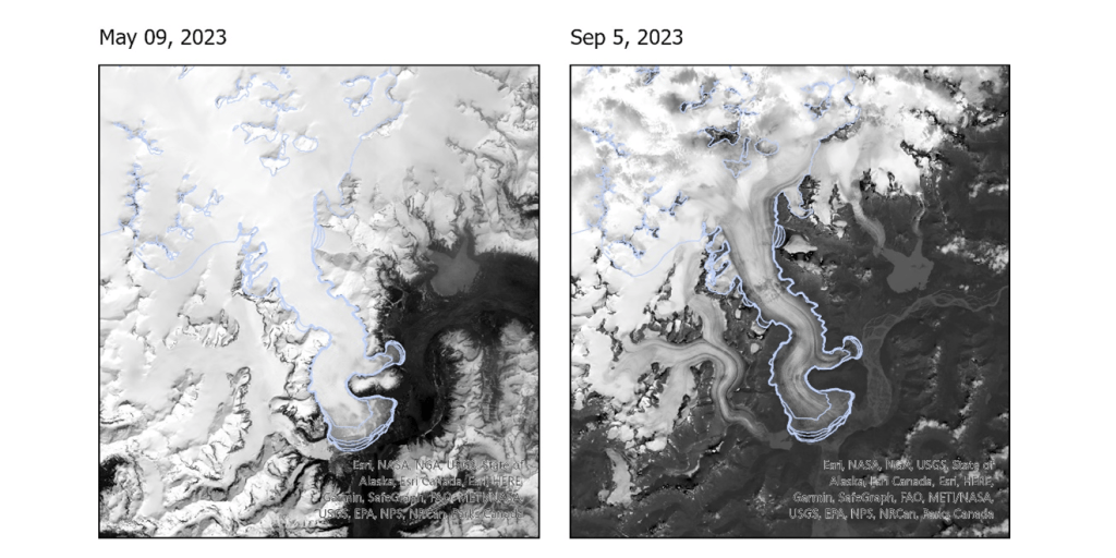
Taku Glacier is shown in two images in Figure 2, which accumulates until the snow stops and temperatures are warm enough for melting in late April to early May. The icefield decreases over summer until it is cold enough for snow to begin falling again, usually by late September or early October. From these images, it is possible to identify the fact that the icesheet thins over the summer, enabling the viewer to visually identify the streaky medial moraines along the middle of the length of the glaciers. Features in the landscape also include terminal moraines at the end of glaciers, as well as the wide braided streams that form as water flows to the Pacific Ocean. These are the features observable on the ground when these glaciers are explored by researchers. An analysis like this is important because it is difficult to visit these sites, and identifying these features remotely can be informative to understand the changes in these regions.

Each map in Figure 3 is the result of a Change Detection analysis as described in the
Methods, and are shown with a partially transparent overlay so some of the underlaying features and topography are visible. In each map, the darker color shows the location where the change is greatest for that wavelength of reflectance. Bands 3 and 5 show the greatest difference in the lower elevation areas near the Taku River. This is as expected, because glaciers usually melt the most at their lower elevation terminus. The increase in reflectance also indicates the increase in vegetation in the now-cleared areas during the summer season. The northern/upper edge has less saturated colors, indicating areas that do not melt through the summer, and do not support vegetation. Band 3 shows that there is increased reflectance due to vegetation in September compared to the reflectance due to vegetation in May. Band 5 indicates increased reflectance overall in may compared to September. The incongruence between these is interesting, and may indicate the data reflect a water-related phenomenon that has not been identified, such as free water on the surface with poorly consolidated or melting precipitation. The map Band 6 (SWIR) illustrates thermal radiation change, and the map demonstrates that there is little variation in the surface temperature of the icefield. Areas that are exposed (not covered with ice or snow) do show different surface temperatures between May and September, and it is this clearing with a resulting change in temperature that is illustrated with Band 6.

There are also interesting features that can be identified in the different bands. For
instance, in Band 3 there is evidence of the braided streams that drain the icefield of water. Band 3 and 5 have stripes that indicate lateral and medial moraines (where debris form striped patterns in the glacier as it flows downhill). Band 6 should be able so “see” through the sparse clouds, but there are a few areas extending from west to east across the middle of the glacier where a few small clouds existed in the September data (and are visible in Figure 2). With this analysis, it is difficult to determine if the clouds are creating a source of error (which indicates a future direction of work), or if the clouds being present has changed the surface temperature.

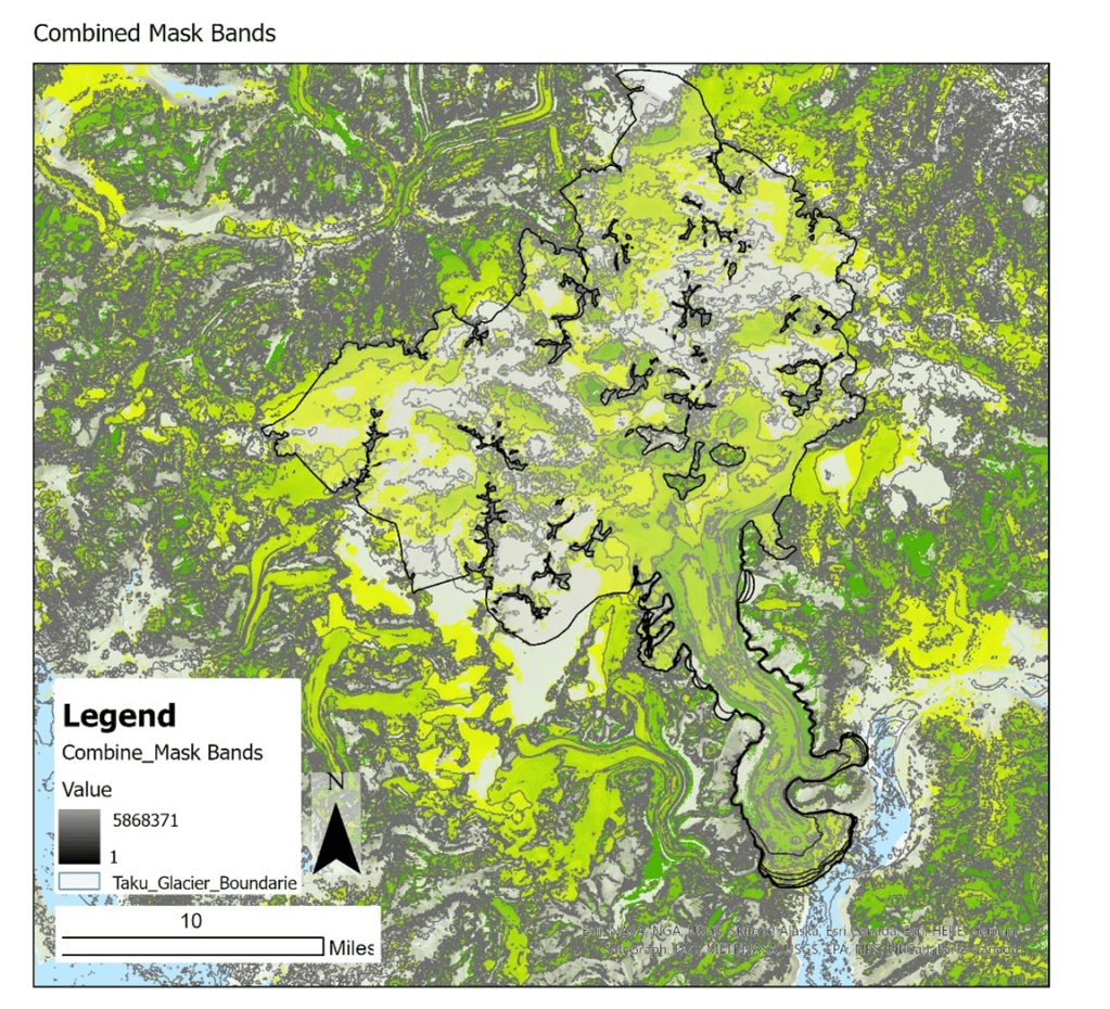
In order to achieve an overall summary of the analysis, the data were combined using the Combine (Spatial Analyst Tool) (Figure 4). This map highlights the points where all the bands are in agreement, and the darkest areas have the most difference from May to September, while the lighter areas have less. As above, this map reinforces the persistence of higher elevation ice (light colors) and the lower elevation shows increased loss of ice (dark color). Additionally, we see the retreat of the glacier from its terminal moraine, and a few higher elevation areas with higher change in ice cover than the adjacent areas.

Conclusions

With this analysis, it is possible to confirm the location of lost ice, and draw it on a map,
which does answer the initial question with a map. Further, it is possible to identify locations where there may be loss of ice that is unexpected or different than the adjacent icefield. Mohanty et al were able to create a model to predict where glacial lakes may form in the Himalaya, but their study did not extend to then mapping glacial lakes that actually formed, in order to validate their method. However, this may be an ongoing project for the research team identified in Mohanty et al as only a single season has passed since their prediction. This study sought to use Landsat data to identify glacial lakes for the purpose of creating a proxy to measure climate effects in a local area. Both prediction and actual measurement are important. In addition to understanding climate change, glacial lakes can become hazards if they threaten to drain suddenly and flood an inhabited area.

For studying the extent of the volume of the icefield, it would improve the result to be able to remove cloud cover from the raster data, so that the dates could be based on the dates of highest and lowest extent of the ice, and were not as heavily influenced by cloud cover. Secondly, it would be interesting to reanalyze this problem perhaps with the same data, but instead of using raster data directly, first using Classification and Recalibration tools to create a custom classification schema, then comparing the classification data to identify the changes to the glacier over time.

Dr. Sarah Fortner (Carleton College) indicated that observations of Taku Glacier in the
summer of 2023 showed that higher elevation glacial lakes formed faster this year than in prior years, which indicates another potential study that would provide more answers and applications for the analysis in this paper. This paper intended to demonstrate that it was possible to use Landsat data to identify the possible locations of these meltwater lakes (or regions), which has been done here. These methods could be applied to other locations, or refined to improve accuracy. However, to test Dr. Fortner’s question, we would need to sample data from multiple years, and then compare the changes for every summer to see if this year was truly atypical.

If I could do this project again, it would be valuable to 1) resolve the issue about clouds and 2) classify and recalibrate the map rather than use the data in a less processed state. A longer term goal would be to create a model or program that could carry out many of the steps of the analysis. Future projects will include looking at the growth of glacial lakes in a prior season, and accessing the difference in glacial lake formation between that season and the 2023 season to determine if the 2023 season was truly atypical.

References

Davies, B., Bendle, J., Carrivick, J., McNabb, R., McNeil, C., Pelto, M., … & Markle, B. (2022). Topographic controls on ice flow and recession for Juneau Icefield (Alaska/British Columbia). Earth Surface Processes and Landforms, 47(9), 2357-2390.

Davies, B., Bendle, J., McNabb, R., Carrivick, J., McNeil, C., Campbell, S., & Pelto, M. (2021, April). Recent, rapid and profound changes to glacier morphology and dynamics, Juneau Icefield, Alaska. In EGU General Assembly Conference Abstracts (pp. EGU21-1539).

Juneau Icefield Research Program. (n.d.). https://juneauicefield.org/
Loyd, C. (2013, June 14). Landsat 8 Bands. NASA Goddard Space Flight Center.
https://landsat.gsfc.nasa.gov/satellites/landsat-8/landsat-8-bands/

Mohanty, L. K., & Maiti, S. (2022). Glacial lake formation probability mapping in the Himalayan glacier: A probabilistic approach. Journal of Earth System Science, 131(1), 54.

U.S. Geological Survey, 2020, Earth Explorer, accessed November 11, 2023 at
URL https://earthexplorer.usgs.gov/

Wolfe, D. F., Kargel, J. S., & Leonard, G. J. (2014). Glacier-dammed ice-marginal lakes of Alaska. In Global land ice measurements from space (pp. 263-295). Berlin, Heidelberg: Springer Berlin Heidelberg.