ON March 11, 2011, an earthquake with a magnitude of 9.0 occurred off the east coast of Japan. The intensity of this earthquake was measured by many monitoring stations.
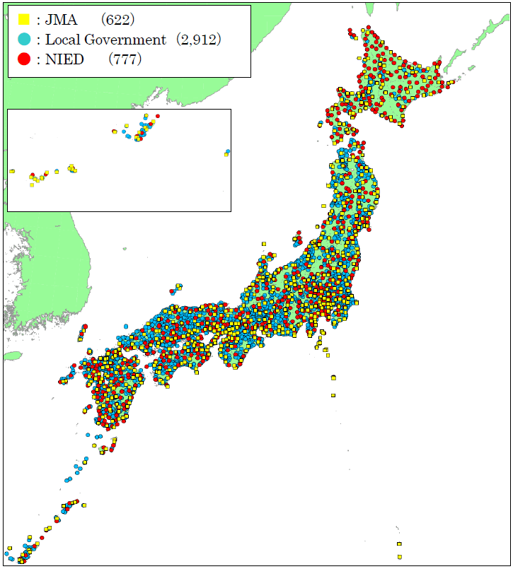
The epicenter of the March 11, 2011 earthquake was located about 45 miles (72 kilometers) east of Tohoku, at a depth of 24 kilometers below the Earth’s surface. This earthquake was followed by over 5,000 aftershocks, with the most significant among them reaching a magnitude of 7.9.
While there are many stations in the region and we are able to collect data about the magnitude of the earthquake across Japan, we can create a map of interpolated data as well. This means we can take data from discrete points, and estimate likely values between the stations where earthquake intensity data was collected.
Interpolation using Inverse Distance Weighted (IDW) is a fundamental data processing technique. IDW interpolation is used to estimate values at un-sampled locations based on the values of surrounding data points. It assumes that values near a particular location are more similar to nearby points than those farther away. The method assigns weights to nearby data points inversely proportional to their distance from the target location, with closer points having a greater influence on the estimate. This results in a smoothed surface or map, making it a valuable tool for various applications such as spatial analysis, environmental modeling, and geostatistics. It’s particularly useful for creating continuous surfaces from discrete point data, aiding in decision-making and understanding spatial patterns.
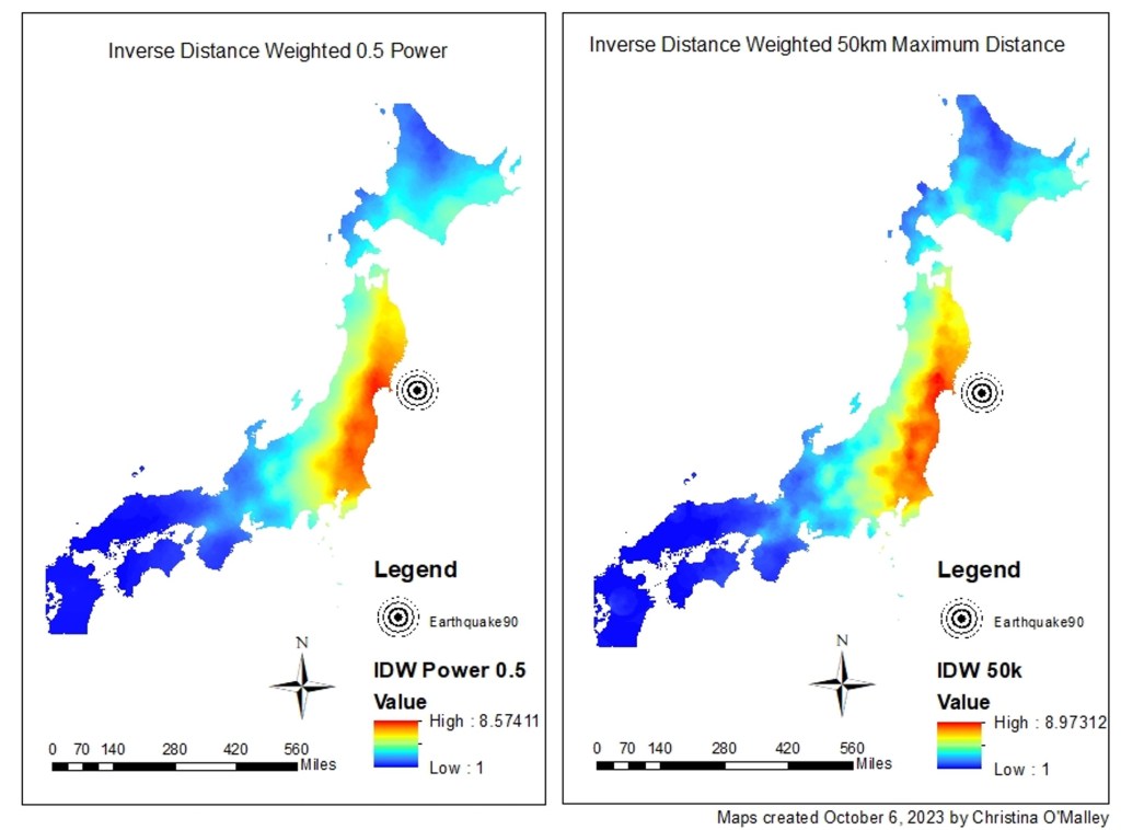
The map on the right (Fig 3a) shows the result when the power is reduced to 0.5 and data is used from the 12 closest values. With this reduction in power, the influence of data on the interpolation of values within cells is reduced. Additionally, using 12 values to calculate interpolated values means that each interpolated value will be influenced by data from a further distance away. The combination of these two variable selections creates a “smoother” surface that shows more gradual changes in cell values.
The map on the left (Fig 13b) shows a IDW analysis with a power of 2 and a 50km maximum distance between 5 of the closest datapoints to each cell. When the power of the IDW is set to 2, each sample point exerts a strong influence on the estimated values of the cells nearby, resulting in a map that is not “smooth”. Additionally, local values have a strong influence as only the 5 closest are used in this analysis (compared to 12 for the map on the left). Having fewer datapoints means that those data each have a larger proportion of influence on the cells that have interpolated values. What we then observe on the map is more variation on a shorter distance, and the map appears to be “less smooth”.
Spline interpolation can estimate values that are below the minimum or above the maximum values found in the sample data. This makes the spline interpolation method good for estimating lows and highs that are not included in the sample data processing.
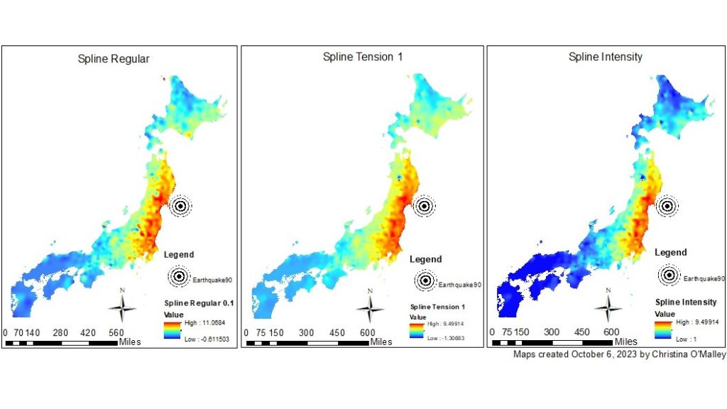
Although this surface does pass through all the sample points, estimates of cell values are influenced more by the direction of change inherent in the data. This means that the estimation of values in adjacent cells is less abrupt, resulting in a surface that appears more continuous and smooth.
SPLINE Regular (Fig 4a) vs SPLINE Tension 1 (Fig 4b)
Regularized spline interpolation may estimate values that depart too much from the sample data. Running a tension spline will flatten out the surface-bending effect (very slightly) around the sample points.
SPLINE Regular (Fig 4a) and Tension 1 (Fig 4b) vs SPLINE Intensity (Fig 4c)
Because the spline interpolation method allows for interpolation below the original values, values less than one are possible. When this occurs, resetting these values to one (the minimum value on the intensity scale) is necessary. You can easily accomplish this by using the Raster Calculator tool to perform a simple if/else evaluation on each of the input cells of an input raster.
 Christina O'Malley, PhD